Sunday, May 6, 2018

Course Content PMP - PMBOK 6

Email : avinesh.singh@gmail.com, 
Mobile:  +91 9701700069
Refer your friend :    To get 20% discount.  
Ask for a demo - Mobile:  +91 9701700069
PMP Training Fee : Rs 9000 (in batch, details below)

Course Details : Following latest syllabus of PMP - PMBOK 6 
I have a very structured and interactive training methodology with innovative presentation done over the internet to help the aspirants to clear the PMP exam in the first attempt. This is an online training, very useful for the aspirants who are working in industries to attend the training from anywhere in the world.
Training by 19 year IT industry management expert

Content Content : 
Through this PMP preparation course I will cover the below chapters from PMBOK6 (latest syllabus for exams starting 26th March 2018).
  1. Introduction to PMP Preparation and Exam Overview
  2. Introduction to Project Management and Fundamental Element
  3. The Environment in which project operates
  4. Role of a Project Manager
  5. Project Integration Management
  6. Project Scope Management
  7. Project Schedule Management
  8. Project Cost Management
  9. Project Quality Management
  10. Project Resource Engagement
  11. Project Communications Management
  12. Project Risk Management
  13. Project Procurement Management
  14. Project Stakeholder Management
In addition to this I will also provide :
  • A pdf covering the chapter notes at the end of  every chapter.
  • Approximately 200 practice questions with their answers. The questions and their answers will be contained in e-books 
  • Analysis of all the important questions of first three chapters.  (Max 25 questions per chapter)
  • At the end of the course I will provide 1400 question and answers to practice before the exam
  • At the end of the course I will provide Guidance to filling up of the PMP application form 
  • Email support for the next 6 months every week end for queries related to the chapters being covered.
  • A certificate of completion with 35 pdu's that you can claim to PMI.
Course Fee :
Rs 9000 - for two members
Rs 12000 - for one to one training
Rs 18000 - for pass guarantee course one to one

Sunday, January 12, 2014

Did you ever understand FINISH TO START, FINISH TO FINISH Task relationships properly ??

Did you ever understand what is Finish-to-Finish, Start-to-Finish or Start-to-Start Task relationships ? Or you are stuck with Finish-to-Start relationship only ?????

Please go through the below post to understand all of the task relationships :

PMBOK® Definition

Logical Relationship: A dependency between two project schedule activities, or between a project schedule activity and a schedule milestone. The four possible types of logical relationships are: Finish-to-Start, Finish-to-Finish, Start-to-Start, and Start-to-Finish. See also precedence relationship.

Precedence Relationship: The term used in the precedence diagramming method for a logical relationship. In current usage, however, precedence relationship, logical relationship, and dependency are widely used interchangeably, regardless of the diagramming method used. See alsological relationship.

Practical Definition

Task relationships determine the start and finish dates of a task as it relates to other activities. The relations are labeled as Finish-to-StartStart-to-Start,Finish-to-Finish and Start-to-Finish.

Expanded Definition

There seems to be relationships in every aspect of life. We have mathematical relationships, money and time relationships, food and wine relationships and even human relationships. So why not project management relationships.

Some relationships are simple while others are complex and baffling. Sometimes they are easier to figure out while others take a bit more noodling. These statements pertain to all relationships and even more so in project management.

Understanding these relationships and their use are critical to the project manager’s success. Why? Because most project managers don’t know they exist, don’t plan properly for their existence, and yet, the relationships exist and happen whether we like it or not.

Once we understand them, know how to apply them and plan according to their natural occurrence, the project schedule more closely reflects the reality of the project. The more closely we model future reality in our plans, the more likely we’ll succeed in our project and meet the stakeholders’ expectations. Additionally, understanding those helps us adjust our efforts and even bend reality at times to bring the project in line with what we want.

Understanding Alphabet Soup: FS, SS, FF, SF

The four relationships are:
  • Finish-to-Start (FS)
  • Start-to-Start (SS)
  • Finish-to-Finish (FF)
  • Start-to-Finish (SF)
Each relationship acts differently as predecessors and successors interact.

Predecessor vs. Successor

PMBOK® Definitions:

Predecessor Activity: The schedule activity that determines when the logical successor activity can begin or end.

Successor Activity: The schedule activity that follows a predecessor activity, as determined by their logical relationship.

Before we can begin to understand the four relationships, we must understand predecessors and successors.

A Predecessor is typically the task that precedes other tasks. Successors typically occur after other tasks, or its predecessors. This is the common understanding of predecessors and successors.

In actuality, predecessors are the tasks that control the relationship between two activities. In fact, predecessors can actually occur after a successor. If that twists your mind a bit, stay with me as I explain how that can happen. I can guarantee you’ve been a victim of activity sequences where the predecessor occurred after its successor.

Finish-to-Start

PMBOK® Definition: The logical relationship where initiation of work of the successor activity depends upon the completion of work of the predecessor activity. See also logical relationship.

Layman’s Definition: Once this task finishes, we can start the next one.

Practical Definition:  In a Finish-to-Start relationship, the predecessor must finish before the successor can start. In fact, the predecessor’s finish date determines the Successor’s start date.

Abbreviation: FS

A Finish-to-Start relationship is typically displayed as follows:


FS is the relationship that occurs the most often within most project schedules. In fact, ninety-five percent (95%) of all tasks are related in a FS relationship. It is the most prevalent of the four relationships. As a result, many project management software packages such as MS Project use it as the default relationship. Unless specified otherwise, the software assumes activities relate in an FS manner.

It basically states once the predecessor finishes, the successor can start.

An example of FS relationships is car washing. We wash the car, dry the car and then wax the car. It makes no sense to dry the car before we wash it. And certainly waxing the car first only grinds the dirt into the paint rather than protecting it.


The activities in car washing naturally fall into a finish-to-start relationship. Of course, we could overlap the activities. In other words, we could start drying the car before we are finished washing it, but we do risk water overspray causing additional necessary drying. The overlapping of activities still follows the definition of finish-to-start relationship because the one spot being dried must be washed and rinsed first.

Start-to-Start

PMBOK® Definition: The logical relationship where initiation of the work of the successor schedule activity depends upon the initiation of the work of the predecessor schedule activity. See also logical relationship.

Layman’s Definition: We want these two tasks to start at the same time.

Practical Definition: Once the predecessor task starts, we can start the successor task.

Abbreviation: SS

A Start-to-Start relationship is typically displayed as follows:


In essence, they all sound the same. The start of the successor task is gated by the start of the predecessor activity. Until the predecessor starts, the successor cannot start.

But here is another meaning people miss. It simply states the successor cannot start UNTIL the predecessor starts. It does not mean it has to start at exactly the same time. It can occur sometime after the beginning of the predecessor’s activity.

An example of a start-to-start relationship might be tabulating results from some market research. In market research, we develop a survey, distribute the survey, and wait for responses to our survey. As we receive the responses, we enter the data into a database and tabulate the information. We do not need to wait for all the responses to return before tabulating the information.

In fact, in market research, a one percent response rate is considered good. Two to four percent response rate is super. But what it really means is we will not receive from 96 to 99% of the desired responses. If we used a finish-to-start relationship between the receiving responses and tabulating the results, we’d never tabulate the responses. Therefore, once the responses flow in, we can start tabulating the results and watch for early trends. This method is what they use during political elections trying to predict the winner before all the votes are counted. Programming this example into project management software would yield the following Gantt chart:


Finish-to-Finish

PMBOK® Definition: The logical relationship where completion of work of the successor activity cannot finish until the completion of work of the predecessor activity. See also logical relationship.

Layman’s Definition: We want these two tasks to finish at the same time.

Practical Definition: Once the predecessor task finishes, the successor task can finish.

Abbreviation: FF

A Finish-to-Finish relationship is typically displayed as follows:

In finish-to-finish relationships, we must wait for the predecessor task to finish before we can finish, or declare, the successor finished. And just as in start-to-start relationships, the successor doesn’t necessarily finish at the same time as the predecessor; it can finish after the predecessor.

When serving dinner, we typically experience, or want to experience, a finish-to-finish relationship. Usually, we want all the food to be ready for eating at the same time and placed on the table, arranged for the family to eat.

Using a finish-to-start relationship while preparing the food results in some portion of the meal cooked while other parts have not even been started. Using a start-to-start relationship while cooking the food can result in some items being over-cooked, under-cooked or just right. Therefore, the only relationship which works for having all the items cooked to the right doneness and placed on the table at the same time is a finish-to-finish relationship.

Let’s say our menu includes meat, potatoes and vegetables. Setting the oven at 350o, the meat takes 45 minutes, the potatoes 60 minutes and the veggies 15 minutes. To properly stage the cooking so all finish at the same time, we would put the potatoes in the oven first, wait 15 minutes, put the meat in, wait another 30 minutes and then add in the vegetables. Programming this example into project management software would yield the following Gantt chart:


Start-to-Finish

PMBOK® Definition: The logical relationship where the completion of the successor schedule activity is dependent upon the initiation of the predecessor schedule activity. See also logical relationship.

Layman’s Definition: This task finishes when the next one starts, but not before then.

Practical Definition: Once the predecessor task starts, the successor task finishes.

Abbreviation: SF

A Start-to-Finish relationship is typically displayed as follows:


Read the definition again. The successor task finishes when the predecessor activity starts. Wait! How can the successor task finish, which means it started, before the predecessor activity starts? I don’t know about you, but this definition twists my brain sideways.

Fortunately, this relationship only occurs less than 1% of the time, so most people miss it, or simply don’t know it exists, but it does. I have seen many people trying to describe this relationship and frankly, most are wrong. So, I provide two here. Don’t go scurrying to the PMBOK for examples because it is conspicuously devoid of examples of these relationships except FS. Hmm…

Imagine you are a dinner boat cruise owner. The boat leaves the dock at 6:00 pm for the cruise around the city. As a smart owner, you open the ticket booth window for sales at 2:00 pm. Your goal is to sell out of all tickets before the boat leaves the dock.

At 5:00 pm, the captain of the boat calls you and says, “Hey boss, I’m stuck in traffic. I’m going to be late. Please let the customers know the boat won’t leave the dock until at least 7:30 pm.”

Six o’clock comes and all the tickets are not sold. As the owner, what do you do? Do you close the ticket sales window and wait for the boat to leave the dock? Do you close the window and go home? Or do you keep selling the tickets until the boat leaves the dock? Of course, you’d keep the window open selling tickets until the cruise is underway.

What determined the finish time of the ticket sales: the clock striking six or the boat leaving the dock? It is the boat leaving the dock. The clock reaching 6:00 pm is meaningless. The boat leaving the dock determines the relationship between the two tasks.

So we see from this example, the predecessor isn’t necessarily the task that comes first, but one that controls the task relationships. If we go back and review the other three relationships already described, we’ll see the same condition – the predecessor determines the relationship. In the start-to-finish relationship, the predecessor is the “main” event, the one determining the finish of the other activity. In the case of the ticket window opening, its opening is determined by the time of day or 2:00 pm. Whether the boat leaves on time or not does not impact the window’s opening.

As we saw, the window’s closing time was extended by the boat’s late departure. Programming this example into project management software would yield the following Gantt chart:


I understand most people reading this definition are not dinner boat cruise owners. So, a more practical example might seat the understanding into memory. Maybe not more practical, but one “closer to home.”

Remember back to the days you went to school. In order to test your knowledge of a subject, the teacher always gave a test. If you were like me, you’d wait until the last minute to cram for the exam. In fact, if the instructor showed up a bit late, you’d still be studying until the test paper hit your desk.

What determined the start of your study time? I never did figure that out, but in my case, it seemed to be panic. But I can tell you what determined the finish of my study time. The professor stating all study material must be put away. That, my fine readers, is a start-to-finish relationship.

Conclusion

Understanding the four relationships between activities in a project schedule helps model reality most accurately. Unfortunately, most project teams only use the finish-to-start relationship between tasks. This method does not accurately schedule the activities of a project.

When planning the steps in a project, actively discuss relationships between all tasks and accurately schedule them. Just as determining the duration of a task is important, relating it to the other things that need to be done is critically important for the success of the project. You might not use all four relationships within a project, but you should at least know they exist and consider them.

Do leave your comments if you enjoy this

Sunday, January 5, 2014

How did a Project come into existence

How did a Project come into existence
Please have a look at the below diagrams that will give you idea on how does a company's Vision, Mission, Business Strategy, Portfolio, Program, Projects and Operations are related.
To understand more : 
Have a look at the PMP TRAINING SUGGESTED BY US


PMP-Difference between Vision and Mission Statement

Difference between Vision and Mission Statement
First a quick summary


About

A Mission statement talks about what the company is now. It concentrates on present; it defines the customer(s), critical processes and it informs you about the desired level of performance.
A Vision statement outlines what a company wants to be. It concentrates on the future; it is a source of inspiration; it provides clear decision-making criteria.

Purpose

A mission statement is spelled out to narrate what the organization is about. It talks about what the company is right now. It lists the broad goals for which the company is formed. It discusses in details what the company does, what the structure is and what its plans are. A vision statement talks about what the company wants to be. It describes what the "vision" of the company is for its future. It lists where the company sees itself some years from now.

Features

Features of an effective vision statement include:
  • Clarity and lack of ambiguity
  • Paint a vivid and clear picture, not ambiguous
  • Describing a bright future (hope)
  • Memorable and engaging expression
  • Realistic aspirations, achievable
  • Alignment with organizational values and culture
  • Time bound if it talks of achieving any goal or objective
Features of an effective mission statement are:
  • Purpose and values of the organization
  • What business the organization wants to be in (products or services, market) or who are the organization's primary "clients" (stakeholders)
  • What are the responsibilities of the organization towards these "clients"
  • What are the main objectives that support the company in accomplishing its mission

Time frame

While a mission statement talks about the present, the vision statement talks about the future. The former mentions what the company is now while the latter describes what the company wants to become in the future. A vision statement mentions what the future will look like for the company if it follows the mission statement.

Developing a statement

When developing a mission statement, it should be seen that the following questions are answered:
  • What do we do today?
  • For whom do we do it?
  • What is the benefit?
When developing a vision statement, it should be seen that the following questions are answered:
  • What do we want to do going forward?
  • When do we want to do it?
  • How do we want to do it?

Which comes first?

For a new start up business, new program or plan to re-engineer your current services, the vision statement will be formulated first as it will guide the mission statement and the rest of the strategic plan.
For an established business where the mission is established, often the mission guides the vision statement and the rest of the strategic plan for the future.
PMP - Difference in the roles of Project and Product Manager

Friday, January 3, 2014

PMP - THE 7 BASIC QUALITY TOOLS

PMP - OTHER TOPICS ->  Difference between Vision and Mission
PMP - OTHE TOPICS -> Difference Product and Project manager

Hi I am Avinesh Singh from http://pmptrack.com

The PMP aspirants would definitely look for a very good explanation of the 7 basic quality tools and their applications. My best efforts to provide you the information from various sources on internet.

MEASURING VARIATION
First I would start with the topic, measuring variation because the quality topic is aligned on meeting the baseline and controlling the variation and identifying or measuring the extent of variation:

I would cover the following :
Understanding variation: Key principles of this important topic.
Measuring variation: Principles of measurement of variation.
Measuring centering: Mean, median and mode.

Measuring spread: Range and standard deviation.


The continuously variable nature of the universe is at the heart of the science of statistics, and at first glance can look very complex, particularly if approached from a mathematical viewpoint. This can lead to it being ignored, which is a pity, as even a simple appreciation of it can result in a reduction in haphazard attempts to control it, with a consequent saving in wasted time and degraded performance.

What is variation?
When a process is executed repeatedly, its outputs are seldom identical. For example, when a gun is successively fired at a target, as in Fig. 1, the bullets will not all pass through the same hole.


Fig. 1. Variation in targeted results

This lack of repeatability is caused by the variation or variability in the process. If these causes are understood, then this can lead to the development of solutions to reduce the variation in the process and result in more consistent products which require less inspection and testing, have less rejection and failure, cost less to build, have more satisfied customers and are more profitable.

Causes of variation
Variation in process output is caused by variations within the process. These may be one or more of:
  1. Differing actions within the process.
  2. Differing effects within the process.
  3. Differing inputs to the process.
As an example for each of these conditions, the variation in the placement of the bullet holes in the target may be affected by:
  1. The gun being held or used differently.
  2. Wear in the hammer mechanism causing the shell to be struck differently.
  3. The bullets being of slightly differing shape or weight.
Thus, even if the first point is eliminated by putting the gun in a clamp and firing it remotely, the bullets will still not all hit the target in the identical position.
The reasons why variation occurs can be divided into two important classes, known as common and special causes of variation. These are discussed further below.

Common causes of variation
Within any process there are many variable factors, as indicated above, each of which may vary a small amount and in a predictable way, but when taken together result in a degree of randomness in the output, as indicated in the figure below. These seemingly uncontrollable factors are called common causes of variation.
Common causes of variation can seldom be eliminated by 'tampering' with the process. For example, consider the effect of simple adjustments to the clamped gun, as in the figure below.


Fig. 2. Tampering

  1. The first hole is to the left of center, so the clamp is rotated a little to the right.
  2. If the clamp had been left alone, the second bullet would have gone a little to the right of center, but as it has been moved right, the bullet now goes further to the right. As a reaction to this, the clamp is rotated somewhat more to the left.
  3. The third bullet tends towards the left anyway, so the result is a hole even further to the left.
It can be seen from this that it would have been better not to tinker with the clamp, and that the score would be more likely to improve if the whole system were understood first and then fundamental improvements made, such as building a better gun or making better bullets.

Special causes of variation
Special causes of variation are unusual occurrences which come from outside the normal common causes, for example where a shot goes outside the main grouping, due to someone tripping over the gunner as the gun is fired, as below:


Fig. 3. Special and common causes of variation

Special causes can thus be addressed as individual cases, finding the cause for each occurrence outside the normal grouping and preventing it from recurring. This may be contrasted with the way that common causes must be addressed through the overall process.
The way that causes are addressed in a process improvement project is usually first to recognize and eliminate special causes, and then to find ways of improving the overall process in order to reduce common causes of variation.
Static and dynamic variation
The distribution of measurements as described above takes no account of time or sequence, as it is not important which measurement came first or last. This isstatic variation.
If the order in which measurements are made is known, then significant trends may be detected, which may be useful for catching a problem before it becomes serious. This is dynamic variation.
For example, if the gunner is initially accurate, but becomes less so as his arm tires, then this may not be detected from the final positioning of holes on the target - it could only be seen by plotting the positioning of the holes across time.
Dynamic variation is commonly measured using the Control Chart.

Measuring variation

Variation is not simple to measure, as by its nature is random and individual events cannot be predicted. Despite this, a degree of measurement can be achieved by looking at how a number of measurements group together. Usually these items are selected with sampling methods.
The spread of measurements within a group enables special causes of variation to be distinguished from common causes of variation. Beyond this, the characteristics of how these random events are spread out can allow improvements in seemingly random chaos to be simply measured.

Distribution of results

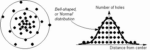
It is common in processes for most measurements to cluster around a central value, with less and less measurements occurring further away from this center. For example, the distribution of holes across the target will gradually spread out from a central, most common placement, as below:


The Normal distribution

The bell-shaped curve in the figure above occurs surprisingly often and is consequently called a Normal distribution (or Gaussian distribution, after its discoverer) and has some very useful properties which can be used to help variation be understood and controlled.

Other distributions

A Normal distribution of measurement values does not always occur, and other distributions may be caused by various factors, conditions and combinations. Several of these are discussed in Chapter 23. It is a trap to use tools that expect a Normal distribution, such as Process Capability, when the distribution is not Normal.

The Central Limit Theorem

The reason for the common occurrence of this Normal distribution is either a natural distribution or the very useful and remarkable effect described by the Central Limit Theorem. This states that, even where the underlying population distribution is not normal, the distribution of the averages of a set of samples will be approximately normal.
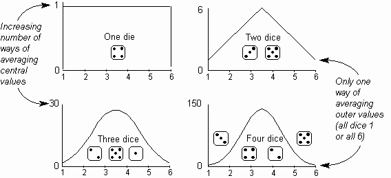
This is clearly illustrated below, which shows the distribution of average values achieved by throwing all possible combinations of one, two, three and four dice.


With a single die, the distribution is rectangular, as there is one, equally likely way of achieving each number. With two dice, the distribution becomes triangular, as although there is only one way of averaging one (two ones), there are six ways of averaging the central value of 3.5 (1-6, 2-5, 3-4, 4-3, 5-2 and 6-1).
With three dice, the distribution becomes curved, and with four dice it is markedly bell-shaped, as there is still only one way of averaging one, but there are four ways of averaging 1.25 (three 1s and a 2) and so on up to 147 ways of averaging 3.5! A key use of this effect is that a predictable Normal distribution can be produced by measuring samples in groups of as few as four items at a time.

Measuring distribution

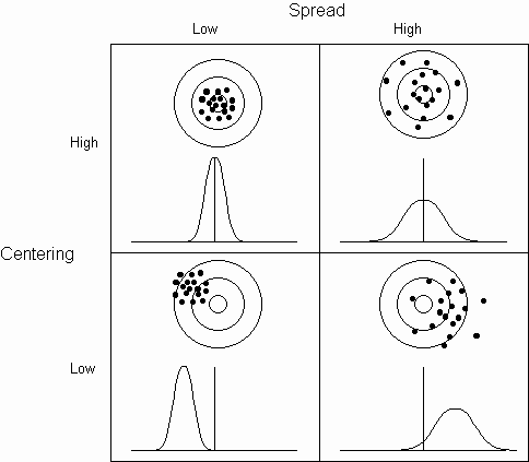
The measurements of a process can vary in two different ways, in terms of their centering and their spread, as illustrated below:
The centering (also called accuracy or central tendency) of a process, is the degree to which measurements gather around a target value. The spread (also calleddispersion or precision) of the process is the degree of scatter of its output values.


Measuring centering

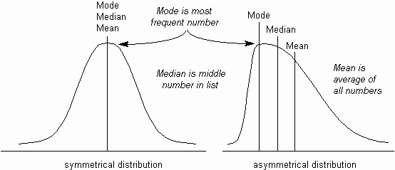
To measure the centering of a process requires that the center point of the set of results be identified. The accuracy of the process can then be determined by comparing it with target values. There are three ways of measuring this center point: the mean (or average), the median and the mode (see the figure below).


Fig. 1. Mean, median and mode in distributions

Mean

The most common way of measuring the center point of a set of measurements is with the average, or mean (i.e. the sum of all measurements divided by the total number of measurements).
The mean is useful for further mathematical treatment, as it considers all values (although a few extreme values can cause the mean to become unrepresentative of the rest of the values).

Median

If the measurements are listed in numeric order, then the median is the number half-way down the list. If there is an even number of measurements, it is half-way between the middle two numbers. The median is not distorted by extreme values, but it can be very unrepresentative of the other values, particularly in a distribution which is not symmetrical.

Mode

The mode is the most commonly occurring measurement. In a distribution graph, this is the highest point. The mode is also not distorted by extreme values, and is useful for measuring such as average earnings. However, there can be more than one mode, and it is not as good as the mean for mathematical treatment.
In a symmetrical distribution such as a Normal distribution, these three measures are the same. In an asymmetrical (or skewed) distribution, as below, there is a simple rule-of-thumb formula which can be used to estimate one, given the other two:
Mean - Mode = 3 x (Mean - Median)

Measuring spread (Range and Standard Deviation)

There are two main ways of measuring the degree of spread of a set of measurements: the range and the standard deviation.

Range

The range of a set of measures is simply the difference between the largest and the smallest measurement value.
Thus, for example, if you have a set of measures (21, 22, 26, 19, 12, 24, 33) then you first find the highest measure (33) and subtract the lowest measure (12) to give the range (21).
This is easy to calculate, but there can be several problems with using it:
  • Special causes of variation can cause an unrealistically wide range.
  • As more measurements are made, it will tend to increase.
  • It gives no indication of the data between its values.

Standard deviation

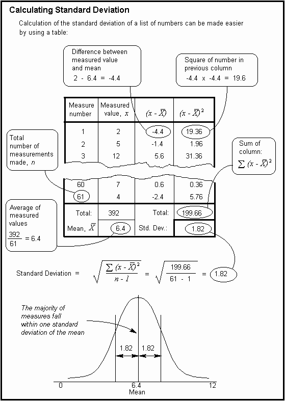
The standard deviation is a number which is calculated using a simple mathematical trick (calculating the square root of the average of squares) to find an 'average' number for the distance of the majority of measures from the mean.
The standard deviation is of particular value when used with the Normal distribution, where known proportions of the measurements fall within one, two and three standard deviations of the mean, as below.


Fig. 1. Percentages in Normal Distribution between Standard Deviations

Thus, given a set of measures, the mean and the standard deviation can be calculated, and from this can be derived the probability of future measures falling into the three bands, provided that the distribution is normal (a simple visual test for this is to draw a histogram and look for the bell shape).
For example, if the gunner has an average score of 56 per target card, with a standard deviation of 6, then, provided the distribution is normal:
  • 68.3% of scores will be 56 ± 6 (= between 50 and 62)
  • 95.4% of scores will be 56 ± 12 (= between 44 and 68)
  • 99.7% of scores will be 56 ± 18 (= between 38 and 74)
or, breaking out the six bands:
  • 2.1% of scores will be between 38 and 44
  • 13.6% of scores will be between 44 and 50
  • 34.1% of scores will be between 50 and 56
  • 34.1% of scores will be between 56 and 62
  • 13.6% of scores will be between 62 and 68
  • 2.1% of scores will be between 68 and 74
  • The remaining 0.3% of scores will be below 38 or above 74.


Hope this was useful